Central Limit Theorem

Last updated on Dec 25, 2022 6 min read

Introduction

We all heard about the Central Limit Theorem (CTL) in out basis statistics class. It is one of the fundamental theorem in statistics and is applied in numerous analytics and statistics analysis. Without any delay, let me state what the theorem says:

Let $X_1, X_2,...., X_n$ be a random sample from a distribution with mean $\mu$ and variance $\sigma^2$. Then if $n$ is sufficiently large, $\bar{X}$ has approximately a normal distribution with $\mu_{\bar{X}} = \mu$ and $\sigma{^2}_{\bar{X}} = \frac{\sigma^2}{n}$. The larger the value of $n$, the better the approximation. The larger the value of $n$, the better the approximation. Devore, J. L. (2000)

Woof, that’s a mathematical definition. Now, let’s break it down in simple words. All that this is saying is that, if we have distribution (any distribution) and draw $n$ samples for $m$ times and plot it’s histogram then, that will resemble to the normal distribution. As a rule of thumb, >30 is a ideal value for the $n$. The below, picture will give you more sense.

The Math Problem

Let’s take a math problem that you may have solved in some statistics class but never realized you utilized the CLT theorem. I am copying this problem from Devore, J. L. (2000).

The amount of a particular impurity in a batch of a certain chemical product is a random variable with mean value 4.0 g and standard deviation 1.5 g. If 50 batches are independently prepared, what is the (approximate) probability that the sample average amount of $\bar{X}$ impurity is between 3.5 and 3.8 g?

The first thing you should note is that, we don’t know which distribution the samples came from. What we know is that, we have 50 batched whose mean is 4 and standard deviation is 1.5. As stated above, 30 is the ideal to use CLT however, here we got 50 so, we should be good to use CLT. One more thing to note is that, the standard deviation is for the means not for the sample. So, we have to calculate the standard error of the mean $(\sigma_{\bar{X}})$ which can be calculated as: $\frac{\sigma}{\sqrt{n}}$

So, to find the probability we can use the properties of normal distribution as the samples satisfies the CLT theorem with the $\mu_{\bar{X}}=4$ and $(\sigma_{\bar{X}}) = \frac{1.5}{\sqrt{50}} = 0.2121$ so,

\[P(3.5 \leq 3.8) = P \left(\frac{3.5-4.0}{.2121} \leq Z \leq \frac{3.8-4.0}{.2121}\right)\] \[ = 0.1645\]

I skipped some steps here. We have the get the respective probability for the Z score and subtract. Since, the main agenda was to understand the problem and realize how CLT is used to solve, I skipped that part. I hope, this gives you more sense. At the start of the problem, we didn’t have idea about the distribution but we solved the problem using CLT. And, that’s the power and beauty of CLT.

The Application

You understood the theorem also solved a math problem and realized it wasn’t that hard. Now let’s take a real life application to better understand the CLT.

The Mushroom Farm Problem

Let’s suppose you are a farmer and you have a big mushroom farm. To give more context, let assume you have 4 farming plots where you have planted about 10,000 mushroom. For simplicity, let’s also assume that all the 4 plots nature is somewhat identical. Meaning, the mushroom are planted on same time, there are same numbers of mushroom planted, they are of same type and they are also exposed to same fertilizers and environment.

Now you are an agriculturist who have an intense background in statistics so wanted to know the probability that the mushrooms on your farms are between some range that will give you maximum profit. If you harvest it early or late, you wouldn’t be able to The simple way to solve this problem is to measure every mushroom on those 4 field, get the data and draw a probability distribution to get the answer. The mushroom farm is visualized below:

However, that solutions have a lot of problems. It is very time consuming and expensive and definitely not feasible. On other hand, the statistical problem is that we don’t know the distribution of the mushroom size so we can’t do any statistics and probability analysis.

Therefore, in such scenario our CLT comes handy.

Solution

So, to find out the probability that our mushrooms are in certain range we can use the CLT. We are going to draw $n$ samples from the Farm 1. Since, we assumed our Farms are same. We also going to take $m$ numbers of samples from the farm. At the end, we will get the $m$ number of means from the Farm 1 sampling.

We will walk through the Python code to understand it workings.


# Import the Libraries
import pandas as pd
import numpy as np
import seaborn as sns
import matplotlib.pyplot as plt

Initially, we said we don’t need to know what distribution the samples comes from and that is still true. However, for the code perspective, I am going to simulate the data points from the exponential distribution. In the function rng.exponential, the first parameter is $\beta = \frac{1}{\lambda}$. Therefore, our $ $. The mean of the exponential distribution is $\lambda$ therefore, the mean of the simulated data points are 1.


# Exponential Distribution or Farm 1 data-points
rng = np.random.default_rng(seed=112233)
exp_dist = rng.exponential(1, 10000)

sns.histplot(exp_dist, kde=True)
plt.title("Simulated Exponential Distribution")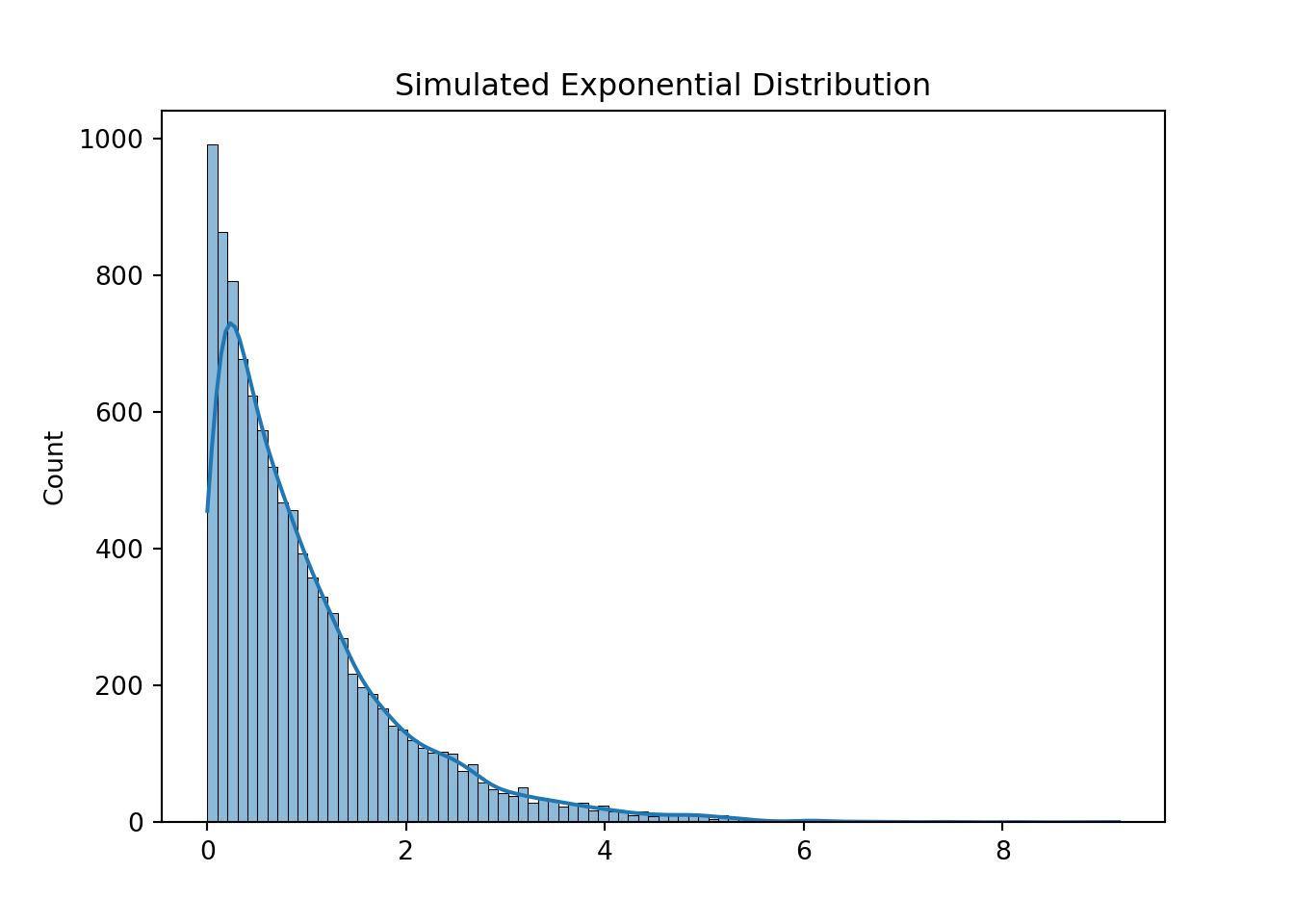

The below sample_mean function calculates the mean of the samples sample_size, up-to n_samples times. So, at the end the function will return the list of the means.


# Sample Mean Calculator function
def sample_mean(distribution_array, sample_size, n_samples):

    # Initialized the list to store value
    sample_mean = []

    for i in range(n_samples):

        # Choose the random samples (Sampling)
        sample = np.random.choice(distribution_array, sample_size,)

        # Calculate the mean of the drawn sample
        mean = np.mean(sample)

        # Append the result
        sample_mean.append(mean)

    return sample_mean

Now, we will draw the graphs of the sample mean distribution for different samples that were drawn from the exponential distribution.


# Plots for different sample sizes
fig, axs = plt.subplots(2,2)
sns.histplot(ax=axs[0,0], x=sample_mean(exp_dist, 1, 500), kde=True)
axs[0,0].set_title("Sample Drawn: 1, 500 Times")
sns.histplot(ax=axs[0,1], x=sample_mean(exp_dist, 10, 500), kde=True)
axs[0,1].set_title("Sample Drawn: 10, 500 Times")
sns.histplot(ax=axs[1,0], x=sample_mean(exp_dist, 30, 500), kde=True)
axs[1,0].set_title("Sample Drawn: 30, 500 Times")
sns.histplot(ax=axs[1,1], x=sample_mean(exp_dist, 50, 500), kde=True)
axs[1,1].set_title("Sample Drawn: 50, 500 Times")
fig.tight_layout()
plt.show()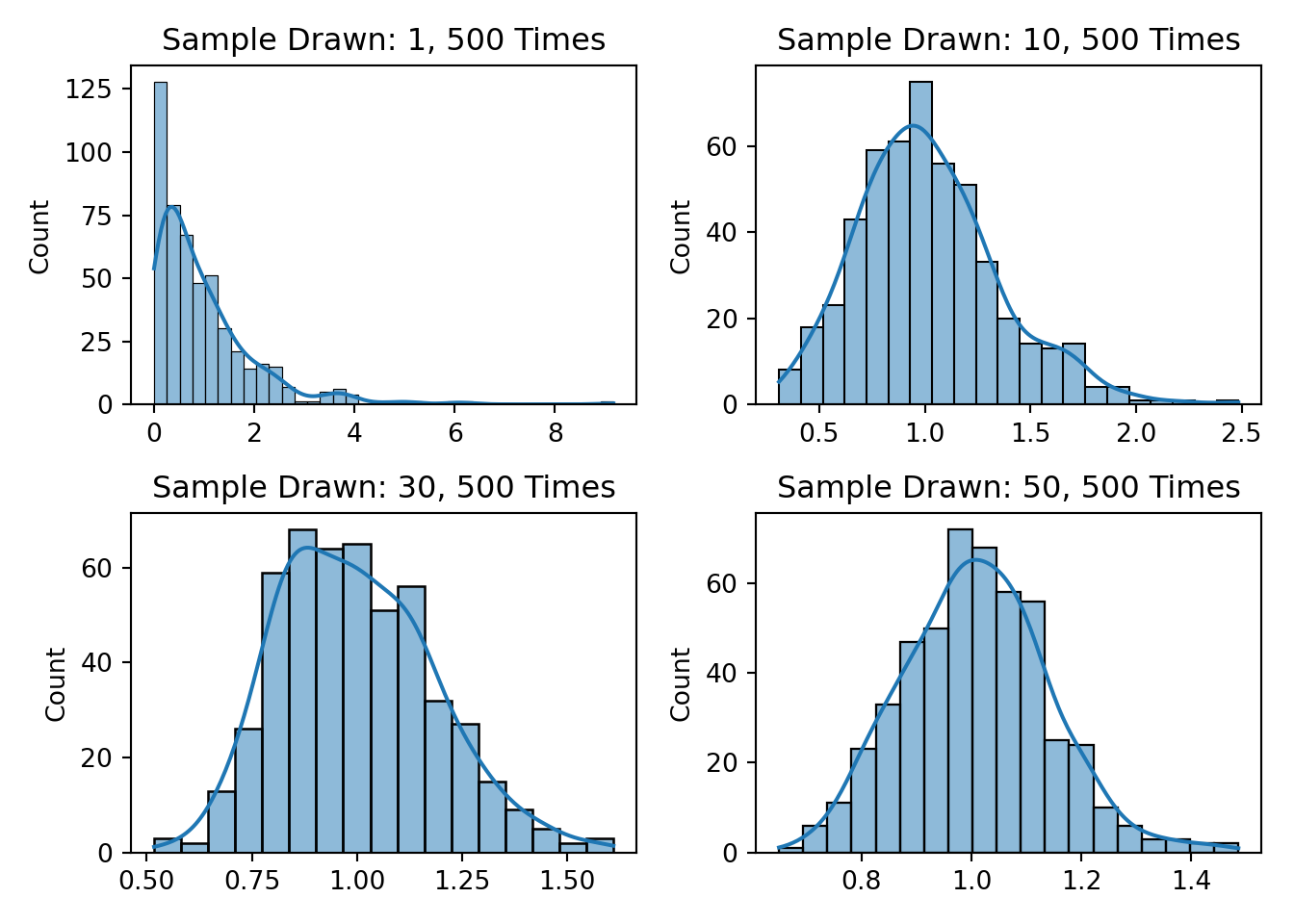

From the above figure, you can clearly see that as we increased the sample size, the distribution is getting closer and closer to normal. With such approximation, we can use the properties of the normal distribution to calculate the various statistics. For example, if we collect large samples like more then 30, we can even do t-test among the different farms even though we don’t have any clue what distribution they follow.

At conclusion, I hope now you have a better understanding of CLT and how it can be used in practice life. I would highly recommend to watch this video if you want to understand from a different application perspective.

References

Devore, J. L. (2000). Probability and statistics for engineering and the sciences (5th ed.). Duxbury.

365 Data Science. (2020, December 21). Real-world application of the Central Limit Theorem (CLT) [Video]. YouTube. https://www.youtube.com/watch?v=N7wW1dlmMaE