Math Behind Linear Regression: Gradient Descent

Gradient descent is one of the most popular optimization algorithms in the data science and machine learning.

For definition, as always, I investigated the Wikipedia. It says, “In mathematics gradient descent (also often called steepest descent) is a first-order iterative optimization algorithm for finding a local minimum of a differentiate function. The idea is to take repeated steps in the opposite direction of the gradient (or approximate gradient) of the function at the current point, because this is the direction of steepest descent.” Now, let me break down the key words from the definition to make ease.

Gradient: Gradient is like a slope. It is the rate of change. The only difference is, slope term is used when there are two variables i.e., x and y, whereas the gradient is applicable in multi-dimensions. Moreover, slope is a scalar whereas gradient is vector

First-Order: It only considers the first derivative when performing the update on the parameter.

Local Minimum: The lowest point of the function. For instance, if the function looks like a parabola facing upward, lowest point is where your function outputs minimum value for a given x.

Differentiable Function: It means we should be able to calculate the derivative of the given function. It sounds obvious. However, if you want to know what kind of function are differentiable, check out this website.

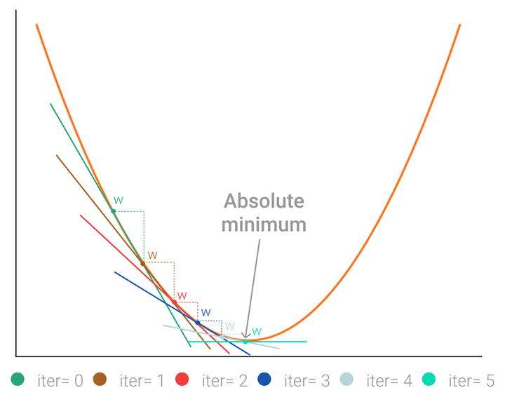
Opposite Direction of Gradient: Since our objective is to find the minimum point, we travel in the opposite direction of the gradient. If we have to reach to the maximum point, we would have travelled in the direction of the gradient.

Iterative: It means finding minimum value by repeating the process until some criteria is met. The criteria can be number of iterations, change is gradient etc. depending upon the problem.

The above whole thing can be summarized by the picture in the top:

Woof, that’s a lot of definition and introduction. Now,let’s move over the application side. We will solve the problem of multiple regression using the Gradient Descent.

First, let’s start with the hypothesis. As we all know the general hypothesis of the linear regression in Ordinary Least Square Method is:

\[ h(x) = \beta_{0} + \beta_{1}x_{1} + \ldots+\beta_{n}x_{n} \tag{1}\] However, we are going to change this equation with different machine learning notation, but the essence remains the same.

\[ h(x) = \theta_{0}x_{0}+\theta_{1}x_{1}+\ldots+\theta_{n}x_{n} \tag{2}\] where \(x_{0} = 1\) and \(x_{1},x_{2},\ldots,x_{n}\) are the multiple input values.

This \(Equation2\) can be changed into the matrix notation which will look like: \[ h_{\theta}(x) = \theta^{T}x \tag{3}\] \(x = [x_{0},x_{1},\ldots,x_{n}]\) and \(\theta = [\theta_{0},\theta_{1},\ldots,\theta_{n}]\)

The whole purpose of the optimization algorithms is to find the optimal value. But what is the optimal situation for the Linear Regression Problem. It is finding the minimum error possible while modeling. In other words, finds the values of \(\theta\) , such that it will give us the lowest error possible.

Now, from the statistics class you may have heard about the Mean Squared Error (MSE). As the word says itself, it is the average of the squared error/residuals. The formula for the MSE is

\[ MSE = \frac{1}{m}\sum_{i=1}^{m}\bigg[h_{\theta}(x^{(i)}) - y^{i} \bigg]^2 \tag{4}\] In the Machine Learning lingo, we call this Loss Function which is modified further:

\[J(\theta_{0},\theta_{1},\ldots,\theta_{n}) = \frac{1}{2m}\sum_{i=1}^m \bigg[h_{\theta}(x^{(i)}) - y^{i} \bigg]^2 \tag{5}\] Now, let’s look at the update rule, meaning how should we change \(\theta\) according to the gradient. As you can see, there is extra constant 2, which is introduced because it makes easier in taking derivatives.

\[ \theta_{j} := \theta_{j} - \alpha \frac{\partial}{\partial\theta_{j}}J(\theta) \tag{6}\] As we see, we introduced a new term \(\alpha\) which is called learning rate. Learning rate is a hyper-parameter for the step size while climbing down the hill. Check this link for more info on learning rate.

For the understanding purpose, let’s first apply the update rule for \(\theta_{0}\) only. The derivative is going to look like:

\[\text{Substituiting eq5 in eq6, we get}\]

\[\theta_{0} = \theta_{0} - \alpha \frac{\partial \bigg(\frac{1}{2m} \sum_{i=1}^{m} \big[h_{\theta}(x^{(i)}) - y^{(i)} \big] \bigg)^2}{\partial \theta_{0}} \]

\[\text{Using Chain Rule}\]

\[\theta_{0} = \theta_{0} - \alpha \bigg(\frac{2}{2m} \sum_{i=1}^{m} \big[h_{\theta}(x^{(i)}) - y^{(i)} \big] \bigg) \partial \frac {(h_{\theta}(x^{(i)}) - y^{(i)})} {\partial\theta_{0}} \]

\[\theta_{0} =\theta_{0} - \alpha \bigg(\frac{1}{m} \sum_{i=1}^{m} \big[h_{\theta}(x^{(i)}) - y^{(i)} \big] x_{0}^{(i)} \bigg) \tag{7}\]

Now, you must be wondering how we went to final step from second last step. Let me break it down for you:

\[ \partial \frac {(h_{\theta}(x^{(i)}) - y^{(i)})} {\partial\theta_{0}} \]

\[\text{From eq2, we can replace the } h_{\theta}(x^{(i)}) \text{ and we will take example for single row only}\]

\[\frac{\partial \big (\theta_{0}x_{0} + \ldots + \theta_{n}x_{n} - y \big)}{\partial \theta_{0}}\]

\[=> x_{0} \]

All part that doesn’t contain \(\theta_{0}\) are constant so, derivative with respect to \(\theta_{0}\) will give zero output.

This is just for the single observation, however for all observation it takes the form of the \(eq7\).

Multiple Linear Regression Using Gradient Descent

The same concept applies to the Multiple Linear Regression. Instead of doing it for only \(\theta_{0}\), we will do it for several variables.

The Gradient descent formula or update rule looks like:

\[ \text{repeat until convergence :}\]

\[\theta_{0} = \theta_{0} - \alpha \bigg(\frac{1}{m} \sum_{i=1}^{m}\big[h_{\theta}(x^{(i)}) - y^{(i)} \big]x_{0}^{(i)} \bigg) \]

\[\theta_{1} = \theta_{1} - \alpha \bigg(\frac{1}{m} \sum_{i=1}^{m}\big[h_{\theta}(x^{(i)}) - y^{(i)} \big]x_{1}^{(i)} \bigg) \]

\[\vdots \]

\[\theta_{n} =\theta_{n} - \alpha \bigg(\frac{1}{m} \sum_{i=1}^{m} \big[h_{\theta}(x^{(i)}) - y^{(i)} \big]x_{n}^{(i)} \bigg)\]

Here, \(\text{repeat untill convergence}\) means updating the \(\theta\)’s until some iteration (epochs) or criteria are reached.

This is just the tip of the Gradient Descent as it has wide application to offer. There are different types of Gradient Descent like Stochastic, Mini-batch which are more popular than the Batch Gradient Descent (Vanilla).

Understanding of Gradient Descent is must in the field of data science/machine learning. I hope this article was helpful to build some intuition behind the working principle. I am not using any code because there are different popular library that does those jobs.

If you want to understand the working of Gradient Descent in Excel, please check out this link

References

Wikimedia Foundation. (2022, February 15). Gradient descent. Wikipedia. Retrieved February 24, 2022, from https://en.wikipedia.org/wiki/Gradient_descent
Géron, A. (2020). Hands-on machine learning with scikit-learn, Keras, and tensorflow: Concepts, tools, and techniques to build Intelligent Systems. O’Reilly.
Mani, A. (2019, December 1). Solving multivariate linear regression using gradient descent. Atma’s blog. Retrieved February 24, 2022, from https://atmamani.github.io/projects/ml/coursera-gd-multivariate-linear-regression/
Gunjal, S. (2020, May 13). Multivariate linear regression from scratch with python. Quality Tech Tutorials. Retrieved February 24, 2022, from https://satishgunjal.com/multivariate_lr/