Logistic Regression
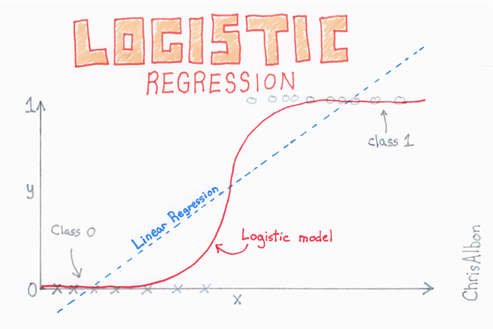 Image credit: Chris Albon
Logistic Regression is one of the most used classification algorithm in statistical analysis and machine learning. The interpretability of output, easy to understand concept and efficient to train makes logistic regression one of the best tool for statistical inference and prediction.
Why not Linear Regression?
The use case of Linear Regression and Logistic Regression is totally different. Linear regression is used to predict continuous set of values whereas logistic regression is used to predict binary prediction like alive or dead, yes or no, 0 or 1 etc. There are techniques to expand the logistic regression to classify multiple classes.
Let us assume we have a dependent variable with binary class 0 and 1 in our dataset. If we use linear regression, some of our estimates might be outside [0,1] interval making them hard to interpret as probabilities.

As shown in the figure above, which I copied from the article in the Medium, we can see the the linear line is not fitting majority of the data points. On the other hand, the best fit line is going above 1 and below 0 making it hard to interpret the target variable. Any time a straight line is fit to a binary response that is coded as 0 or 1, the prediction can always get probabilities <0 or for some values and >1 for some values.
Let us define \(P(X)\) be the linear regression function which is defined as \(P(X) = \beta_{0}+\beta_{1}X\), where \(\beta_{0}\) and \(\beta_{1}\) are the coefficients of intercept and independent variable respectively.
Now, to restrict the functions output between 0 and 1 for all values of \(X\), we will use logistic function which will restrict the output within the range [0,1].
\[P(X) = \frac{e^{\beta_{0}+\beta_{1}X}}{1+e^{\beta_{0}+\beta_{1}X}} \tag{1}\] When further simplified by cross-multiplication and taking common, we will end up with
\[\frac{P(X)}{1-P(X)}= e^{\beta_{0}+\beta_{1}X} \tag{2}\]
The left-hand side of the equation is called odds and can take any value between 0 and \(\infty\). According to the dictionary Merriam-Webster, Odds simply means the probability that one thing is so or will happen rather than another. The value of odds close to 0 indicated low probabilities whereas high value indicated high probabilities.
By taking \(\log\) on both sides of the above equation:
\[\log\left({\frac{P(X)}{1-P(X)}}\right)= \beta_{0}+\beta_{1}X \tag{3}\] The left-hand side is called the log-odds or logit. We see that logistic regression model has a logit that is linear in \(X\). In linear regression \(\beta{1}\) gives the change rate in \(Y\) with one unit increase in \(X\). However, in logistic regression, increasing \(X\) by one unit change log odds by \(\beta_{1}\).
Since, the hurdle to restrict the value within 0 and 1 is solved, we now proceed to find the value of our coefficients.
Finding the Coefficients
The coefficients are estimated based on the training data with mathematical equation called likelihood function. I am not going to explain this function in detail and which is also not necessary at the moment. One doesn’t have to write the function and work from bottom up, R does the stuff for you. However, I will lay down the function below:
\[l(\beta_{0}, \beta_{1}) = \prod_{i:y_{i}=1} p(x_{i}) \prod_{i^{\prime}:y_{i^{\prime}}=0} (1-p(x_{i^{\prime}})) \tag{4}\]
Let’s Predict
After finding the \(\beta_{0}\) and \(\beta_{1}\), we simply plug the value of \(X\) for the needed prediction. We will use the logit function which is our equation 1. Since, \(\beta_{0}\) and \(\beta_{1}\) are estimated by the likelihood function, we plug the dependent variable i.e. X which will give us the respective probability of that instance.
The same idea can be expanded for the multiple independent variables. For the categorical variables, the data is encoded as dummy variable. Moreover, Logistic Regression can also used to classify a response variable that has more than two classes.
Demo
In this section, I will demonstrate the working process of logistic regression in R.
#Installing the package
suppressPackageStartupMessages(library(tidyverse))            #for data manipulation
suppressPackageStartupMessages(library(ISLR))                 #for dataset
## Warning: package 'ISLR' was built under R version 4.0.5#Importing Dataset
data("Default") #dataset#Summerizing the data
summary(Default)## default student balance income
## No :9667 No :7056 Min. : 0.0 Min. : 772
## Yes: 333 Yes:2944 1st Qu.: 481.7 1st Qu.:21340
## Median : 823.6 Median :34553
## Mean : 835.4 Mean :33517
## 3rd Qu.:1166.3 3rd Qu.:43808
## Max. :2654.3 Max. :73554We can see that, there are 3 independent variable and our dependent variable is default which has two classes ‘Yes’ and ‘No’. The total data points are 10,000. For more info, on the dataset go to this link and access the reference manual.
#Building Model
model <- glm(default~., family="binomial", data=Default)
summary(model)
##
## Call:
## glm(formula = default ~ ., family = "binomial", data = Default)
##
## Deviance Residuals:
## Min 1Q Median 3Q Max
## -2.4691 -0.1418 -0.0557 -0.0203 3.7383
##
## Coefficients:
## Estimate Std. Error z value Pr(>|z|)
## (Intercept) -1.087e+01 4.923e-01 -22.080 < 2e-16 ***
## studentYes -6.468e-01 2.363e-01 -2.738 0.00619 **
## balance 5.737e-03 2.319e-04 24.738 < 2e-16 ***
## income 3.033e-06 8.203e-06 0.370 0.71152
## ---
## Signif. codes: 0 '***' 0.001 '**' 0.01 '*' 0.05 '.' 0.1 ' ' 1
##
## (Dispersion parameter for binomial family taken to be 1)
##
## Null deviance: 2920.6 on 9999 degrees of freedom
## Residual deviance: 1571.5 on 9996 degrees of freedom
## AIC: 1579.5
##
## Number of Fisher Scoring iterations: 8In the model building glm() function, we started with the y value (dependent variable) connecting all dependent variable(Note: If you want to use all the columns of your data frame then just put period sign like in above code.) by tilde(~) sign. We put ‘binomial’ on the ‘family’ because we are using logistic regression.
The summary output throws a bunch of useful information. The coefficients section give the estimated \(\beta\) for the respective variable with the p-value for the significance. Let me remind you one more time, the coefficient is log odds. It is explained as, one unit increase in ‘balance’ is associated with an increase in log odds of default by 0.0057.
#Predicting the value
predict(model,newdata=data.frame(student="No",balance=1000,income=50000), type="response")
## 1
## 0.006821253So, we predicted the probability of the new data that we fed into the ‘predict()’ function. In the function, first we have our model, newdata and type. The ‘type’ tells that we want our answer in probability. From the code, we got our predicted probability as 0.68%, which is pretty low. So, we can conclude that this instance is most likely to get a ‘No’. Generally, the cutoff value for ‘Yes’ & ‘No’ is 50%, however this can be changed depending upon the problem.
In this demo, I am skipping various steps. Some of them are, splitting the data into train & test data to calculate the accuracy and efficiency of the model, confusion matrix, cross-validate, detailed EDA etc. The sole purpose of the article is to give you some basic theoretical concept of Logistic Regression and interpretation of results when analysis is done in R.
At last, if one wants to master data science, machine learning, or any analysis, logistic regression is a must known algorithm.
Note: For the article, I was dependent upon “An Introduction to Statistical Learning” book. This is by far one of the best book on getting started with data science. I highly advise to read the book.