Are we SMOTING correctly?
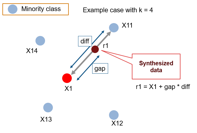 Photo by Analytical Vidhya
The class imbalance problem is very common scenario that we encounter in various domains like Churn Analysis in HR, Fraud Analysis in Finance, Customer Retention in Marketing. Class Imbalance simply means that in our multi-class target variable the proportion are not equally close to each other. For instance, in dichotomous classification problem to find fraudulent transactions our data might have 10 fraudulent transactions out of 100, which is very common, considering the nature of the problem. So, in simple terms, there are more observation for one class as compared to another.
Now, the question is why class imbalance is a problem in data science and what are its effects? As, we all know, the core working principle of the any classification algorithm is to find a decision boundary to separate the two class (I will take binary classification as default in all part of the blog). The algorithms learn from the data to find the optimal boundary. When we have more observations on one class, our algorithms identify the pattern for that majority class but not for the minority class. Therefore, the algorithms learn various pattern for the majority class and might perform well for that one. However, on the other hand, for minority class, it will struggle.
There are various techniques to mitigate the class-imbalance problem. Some of them are Oversampling, Under-Sampling, Cost-Sensitive Algorithms, SMOTE (Synthetic Minority Over-Sampling Techniques) (Chawla et al., 2002). In this blog, we will particularly talk about the SMOTE which is probably one of the widely used techniques in resolving the class-imbalance problem. I am specifically going to talk about the procedure, the common mistakes, and pitfalls as well as the right way to SMOTE.
I will implement all the process in Python. So, let’s get started.
Import the Libraries
import pandas as pd
import numpy as np
import matplotlib.pyplot as plt
from imblearn.datasets import fetch_datasets
from collections import Counter
from sklearn.model_selection import train_test_split
from sklearn.linear_model import LogisticRegression
from imblearn.over_sampling import SMOTE
from sklearn.metrics import roc_auc_score
from sklearn.metrics import classification_report
from sklearn.metrics import confusion_matrix
from sklearn.metrics import ConfusionMatrixDisplay
from imblearn.under_sampling import RandomUnderSampler
from imblearn.pipeline import Pipeline
Load the dataset
In this blog, we will utilize the Abalone Data Set that can be found at this link on UCI website. It is also pre-attached to the imblearn package, so we will fetch from the api itself.
# Get the 'Abalone' Data
df = fetch_datasets()["abalone"]

# Seperate the feature and target
X, y = df.data, df.target

# Count the target-class
print(Counter(y))
## Counter({-1: 3786, 1: 391})From the above output, you can see that there are two classes [-1,1] and we can clearly see the imbalance targets.
We will then divided the data into train-test set for validation and evaluation.
Train-Test Split
X_train, X_test, y_train, y_test = train_test_split(X, y, train_size=0.8,
                                  stratify=y, random_state=112233)
Pitfall Alert: One of the common mistakes, we all do is not to
stratify the train and test set. In the balanced dataset, it wouldn’t
matter but in imbalance dataset it will have profound impact. If we
enable the stratify in the train_test_split function, it will keep
the same proportion of the classes in the both train and test set. This
stratification gives the unbiased split for training as well as testing.
Let’s verify that by checking the proportion of the test and train set.
train_counter = Counter(y_train)
train_prop = [(i, train_counter[i]/len(X_train) * 100) for i in train_counter]
print(f"The train data prop: {train_prop}")
## The train data prop: [(-1, 90.63154744088597), (1, 9.368452559114038)]test_counter = Counter(y_test)
test_prop = [(i, test_counter[i]/len(X_test) * 100) for i in test_counter]
print(f"The test data prop: {test_prop}")## The test data prop: [(-1, 90.66985645933015), (1, 9.330143540669857)]Logistic Regression (No SMOTE)
First of all, we will train the model without SMOTE so that we can compare and contrast the effect of SMOTE on the results. I choose to go along with Logistic Regression (LR) as it is one of the famous and easy to understand. However, the purpose of the blog is to compare the result difference before and after SMOTE, not the modeling algorithm. You can try with another one to experiment on your own.
lr_noSmote = LogisticRegression(random_state=112233).fit(X_train, y_train)Logistic Regression (With SMOTE)
SMOTE
Pitfall Alert: In some of the class project, I have witnessed a basic problem while performing SMOTE. They applied the SMOTE on the whole dataset. You should only apply SMOTE after splitting the dataset, not on the whole raw dataset. Otherwise, we have a problem of the data-leakage. So, make sure you only apply the SMOTE or any other sampling techniques to the split train set.
There and various sampling_strategy in the SMOTE function while
oversampling the minority class. I have used the sampling_strategy as
0.3 which means the minority and the majority proportion after smoting
will be the 0.3. Please, refer to the imblearn api for more detailed
explanation on different sampling_strategy. I choose 0.3 arbitrarily
however, for optimal modeling we can tune this parameter and see what
gives us better performance.
sm = SMOTE(random_state=112233, sampling_strategy=0.3)
X_res, y_res = sm.fit_resample(X_train, y_train)

print('Original Data: ', Counter(y_train))
## Original Data: Counter({-1: 3028, 1: 313})print('Smoted Data: ', Counter(y_res))## Smoted Data: Counter({-1: 3028, 1: 908})Model
We are fitting the Logistic Regression model with our resampled data.
lr_smote = LogisticRegression(random_state=112233).fit(X_res, y_res)Comparing the SMOTE and NON-SMOTE model
Let’s bring the two models to the battle-ground and see if there is any improvements. We will use the ROC-AUC score to compare different models. It is advised for imbalance dataset accuracy is not the right metric as it can be biased and gave false interpretation.
# No-SMOTE model
y_pred_nosmote = lr_noSmote.predict(X_test)


print('Accuracy (No Smote): ',lr_noSmote.score(X_test, y_test))
## Accuracy (No Smote): 0.9066985645933014print('AUC Score (No Smote): ', roc_auc_score(y_test, y_pred_nosmote))## AUC Score (No Smote): 0.5print('Confusion Matrix (No Smote): ', "\n",confusion_matrix(y_test, y_pred_nosmote,
labels=lr_noSmote.classes_), '\n')
# SMOTE Model## Confusion Matrix (No Smote):
## [[758 0]
## [ 78 0]]y_pred_smote = lr_smote.predict(X_test)
print('Accuracy (SMOTE): ',lr_smote.score(X_test, y_test))## Accuracy (SMOTE): 0.8576555023923444print('AUC Score (SMOTE): ',roc_auc_score(y_test, y_pred_smote))## AUC Score (SMOTE): 0.6167207902036398print('Confusion Matrix (SMOTE): ', "\n", confusion_matrix(y_test, y_pred_smote,
labels=lr_smote.classes_))
## Confusion Matrix (SMOTE):
##  [[692  66]
##  [ 53  25]]
From the above comparison, we can clearly see that the model where SMOTE is applied performed better then the without SMOTE one. We have increased the AUC score as well as we have also correctly classified more number of minority class. In the plain data, we correctly classified the majority class but our model couldn’t separate any of the minority class. On the other hand, the SMOTED model, was able to separate 25 minority class in expense of majority class errors.
Pitfall Alert: Don’t compare the model performance with accuracy metric for the imbalanced dataset. Our SMOTED model’s accuracy has decreased but that doesn’t mean the model isn’t better then the plain model. Let’s take the same example of the our fraudulent detection. If we implement plain model like above we identified all the non-fraudulent activity but none of the fraudulent activity. Does that solve our main problem which is to identify fraudulent activity? Absolutely No. However, the SMOTED model is able to identify more fraudulent activity as compared to plain one. So, which model will you choose for production? I am sure you all are deviated towards the SMOTED one.
Now, will you be surprised if I tell you that is not the right way to SMOTE? Then, get ready to be surprised.
SMOTE: The Right Way
In the original paper by Chawla et.al (2002), they performed their comparision by combining oversampling with SMOTE and then under-sampling the majority class. However, in many of the paper and projects, what I have seen is that most of them have only used over-sample with SMOTE but haven’t done under-sample.
In the below also, the over-sampling strategy remains the same - 0.3. In the under-sample, I choose the strategy to be 0.5 meaning, the ratio of majority and minority will be 0.5. Our new mixed method will have fewer data-points then the SMOTED model because we under-sampled after the SMOTE.
# Over-Sample
os = SMOTE(random_state=112233, sampling_strategy=0.3)

# Under-Sample
us = RandomUnderSampler(random_state=112233, sampling_strategy=0.5)

# Pipeline
pipe = Pipeline(steps = [('over', os), ('u', us)])

# New train Dataset
X_mix, y_mix = pipe.fit_resample(X_train, y_train)

# Count of the new data
print(Counter(y_mix))

# Modeling
## Counter({-1: 1816, 1: 908})lr_mix = LogisticRegression(random_state=112233).fit(X_mix, y_mix)
# Prediction
y_pred_mix = lr_mix.predict(X_test)
# Metrices
print('Accuracy: ',lr_mix.score(X_test, y_test))## Accuracy: 0.812200956937799print('AUC Score: ',roc_auc_score(y_test, y_pred_mix))## AUC Score: 0.7181685948176714print('Confusion Matrix: ',"\n",confusion_matrix(y_test, y_pred_mix, labels=lr_mix.classes_))## Confusion Matrix:
## [[632 126]
## [ 31 47]]Below is the table that compare the plain, smoted and mixed model result:
| Model | AUC Score | Correctly Classified Minority Class |
|---|---|---|
| Plain | 0.5 | 0/78 |
| SMOTE only | 0.61 | 25/78 |
| SMOTE + Under-Sample | 0.81 | 47/78 |
As you can see from the result, our dataset is decreased. However, with this fewer data points also, we have substantial increased the AUC score. The model was able to classify more minority class. So, it is clear that over-sample with SMOTE followed by under-sample performs better. I want to reiterate that the test data are same across all the models that we compared. So, why this works? I am copying the answer from the original paper, “Our method of synthetic over-sampling works to cause the classifier to build larger decision regions that contain nearby minority class points.”.
Final Notes
- Extension of the SMOTE
There are various extension of SMOTE that works on the variety of
dataset. For the dataset containing mix of categorical and numeric
variable there is SMOTE-NC. I would suggest to look at the imblearn
official API for more variety and apply the extension that fits your
scenario.
- SMOTE in Real-World Application
In the recent paper by Tarawneh et al.(2022), they empirically showed that the variety of over-sampling techniques including SMOTE and it’s extensions, are deceptive and could lead to severe failure in real-world application. They found that, when the datasets were changed it produced intolerable number of errors.
- Is SMOTE needed?
One study by Elor & Averbuch-Elor (2022) demonstrated that balancing with SMOTE could be beneficial for the weak classifier but not for the strong ones. This means, we might see some improvements in the results with SMOTE if applied to simpler algorithms like Logistic Regression, Decision Tree, Naive Bayes but we might not see those improvement if ensemble or complex algorithms like Catboost, XGBoost etc are used. In their experiment, the Catboost without balancing outperformed the balanced one.
So, should we use SMOTE? The answer is, “it depends”. As answer to many Data Science question, we have to experiment and see how it reacts to our scenario. Experiment with different methods and see what gives you optimal result.
References
Chawla, N. V., Bowyer, K. W., Hall, L. O., & Kegelmeyer, W. P. (2002). SMOTE: Synthetic minority over-sampling technique. Journal of Artificial Intelligence Research, 16, 321–357. https://doi.org/10.1613/jair.953
Elor, Y., & Averbuch-Elor, H. (2022). To SMOTE, or not to SMOTE? Arxiv.Org. http://arxiv.org/abs/2201.08528
Tarawneh, A. S., Hassanat, A. B., Altarawneh, G. A., & Almuhaimeed, A. (2022). Stop Oversampling for Class Imbalance Learning: A Review. IEEE Access, 10, 47643–47660. https://doi.org/10.1109/ACCESS.2022.3169512